Bayesian inference is distinguished by a broad view of probability, not by the use of Bayes’ theorem.
Scientific inference is often framed as follows:
- An hypothesis is either true or false;
- we use a statistical procedure and get an imperfect cue of the hypothesis’ falsity;
- we (should) use Bayes’ theorem to logically deduce the impact of the cue on the status of the hypothesis. It’s the third step that is hardly ever done.
3.2. Sampling to summarize
Common questions to ask using posterior probabilities are divided into questions about (1) intervals of defined boundaries, (2) questions about intervals of defined probability mass, and (3) questions about point estimates.
3.2.1. Intervals of defined boundaries
How much posterior probability lies between 0.5 and 0.75?
# define grid
p_grid <- seq(from = 0, to = 1, length.out = 1000)

# define prior
prior <- rep(1, 1000)

# compute likelihood at each value in grid
likelihood <- dbinom(6, size = 9, prob = p_grid)

# compute product of likelihood and prior
posterior <- likelihood * prior

# standardize the posterior, so it sums to 1
posterior <- posterior / sum(posterior)

# sample the posterior
samples <- sample(p_grid, prob = posterior, size = 1e4, replace=TRUE)

# ask a question
sum(samples > 0.5 & samples < 0.75) / 1e4
## [1] 0.61323.2.2. Intervals of defined mass
It is more common to see scientific journals reporting an interval of defined mass, usually known as a confidence interval. An interval of posterior probability, such as the ones we are working with, may instead be called a credible interval. These posterior intervals report two parameter values that contain between them a specified amount of posterior probability, a probability mass.
When intervals assign equal probability mass to each tail, they are known as percentile intervals (PI). For example, where are the boundaries of the 80% percentile confidence interval?
quantile(samples, c(0.1, 0.9))## 10% 90%
## 0.4483483 0.8108108These intervals do a good job of communicating the shape of a distribution, as long as the distribution isn’t too asymmetrical. But in terms of supporting inferences about which parameters are consistent with the data, they are not perfect.
To overcome this, we can use the highest posterior density interval (HPDI).
If you want an interval that best represents the parameter values most consistent with the data, then you want the densest of these intervals The HPDI is the narrowest interval containing the specified probability mass.
rethinking::HPDI(samples, prob = 0.8)## |0.8 0.8|
## 0.4744745 0.8308308The HPDI also has some disadvantages. HPDI is more computationally intensive than PI and suffers from greater simulation variance, which is a fancy way of saying that it is sensitive to how many samples you draw from the posterior. It is also harder to understand and many scientific audiences will not appreciate its features, while they will immediately understand a percentile interval, as ordinary non-Bayesian intervals are nearly always percentile intervals (although of sampling distributions, not posterior distributions).
Overall, if the choice of interval type makes a big difference, then you shouldn’t be using intervals to summarize the posterior. Remember, the entire posterior distribution is the Bayesian estimate. It summarizes the relative plausibilities of each possible value of the parameter. Intervals of the distribution are just helpful for summarizing it. If choice of interval leads to different inferences, then you’d be better off just plotting the entire posterior distribution.
Why 95%? The most common interval mass in the natural and social sciences is the 95% interval. This interval leaves 5% of the probability outside, corresponding to a 5% chance of the parameter not lying within the interval. This customary interval also reflects the customary threshold for statistical significance, which is 5% or p < 0.05. It is not easy to defend the choice of 95% (5%), outside of pleas to convention. Often, all confidence intervals do is communicate the shape of a distribution. In that case, a series of nested intervals may be more useful than any one interval. For example, why not present 67%, 89%, and 97% intervals, along with the median? Why these values? No reason. They are prime numbers, which makes them easy to remember. And these values avoid 95%, since conventional 95% intervals encourage many readers to conduct unconscious hypothesis tests.
What do confidence intervals mean? It is common to hear that a 95% confidence interval means that there is a probability 0.95 that the true parameter value lies within the interval. In strict non-Bayesian statistical inference, such a statement is never correct, because strict non-Bayesian inference forbids using probability to measure uncertainty about parameters. Instead, one should say that if we repeated the study and analysis a very large number of times, then 95% of the computed intervals would contain the true parameter value. But whether you use a Bayesian interpretation or not, a 95% interval does not contain the true value 95% of the time. The history of science teaches us that confidence intervals exhibit chronic overconfidence. The 95% is a small world number, only true in the model’s logical world. So it will never apply exactly to the real or large world.
3.2.3. Point estimates
In order to decide upon a point estimate, a single-value summary of the posterior distribution, we need to pick a loss function. Different loss functions nominate different point estimates. The two most common examples are the absolute loss \(|d - p|\), which leads to the median as the point estimate, and the quadratic loss \((d - p)^2\), which leads to the posterior mean as the point estimate.
3.3. Sampling to simulate prediction
Another common job for samples from the posterior is to ease simulation of the model’s implied observations. Generating implied observations from a model is useful for at least four distinct reasons:
- Model checking. After a model is fit to real data, it is worth simulating implied observations, to check both whether the fit worked correctly and to investigate model behavior.
- Software validation. In order to be sure that our model fitting software is working, it helps to simulate observations under a known model and then attempt to recover the values of the parameters the data were simulated under.
- Research design. If you can simulate observations from your hypothesis, then you can evaluate whether the research design can be effective. In a narrow sense, this means doing power analysis, but the possibilities are much broader.
- Forecasting. Estimates can be used to simulate new predictions, for new cases and future observations. These forecasts can be useful as applied prediction, but also for model criticism and revision.
Bayesian models are always generative, capable of simulating predictions.
3.3.2. Model checking
Model checking means (1) ensuring the model fitting worked correctly and (2) evaluating the adequacy of a model for some purpose. Since Bayesian models are always generative, able to simulate observations as well as estimate parameters from observations, once you condition a model on data, you can simulate to examine the model’s empirical expectations.
After assessing whether the posterior distribution is the correct one, because the software worked correctly, it’s useful to also look for aspects of the data that are not well described by the model’s expectations. The goal is not to test whether the model’s assumptions are “true,” because all models are false. Rather, the goal is to assess exactly how the model fails to describe the data, as a path towards model comprehension, revision, and improvement.
We’d like to propagate the parameter uncertainty—carry it forward—as we evaluate the implied predictions. All that is required is averaging over the posterior density for p, while computing the predictions. For each possible value of the parameter p, there is an implied distribution of outcomes. So if you were to compute the sampling distribution of outcomes at each value of p, then you could average all of these prediction distributions together, using the posterior probabilities of each value of p, to get a posterior predictive distribution.
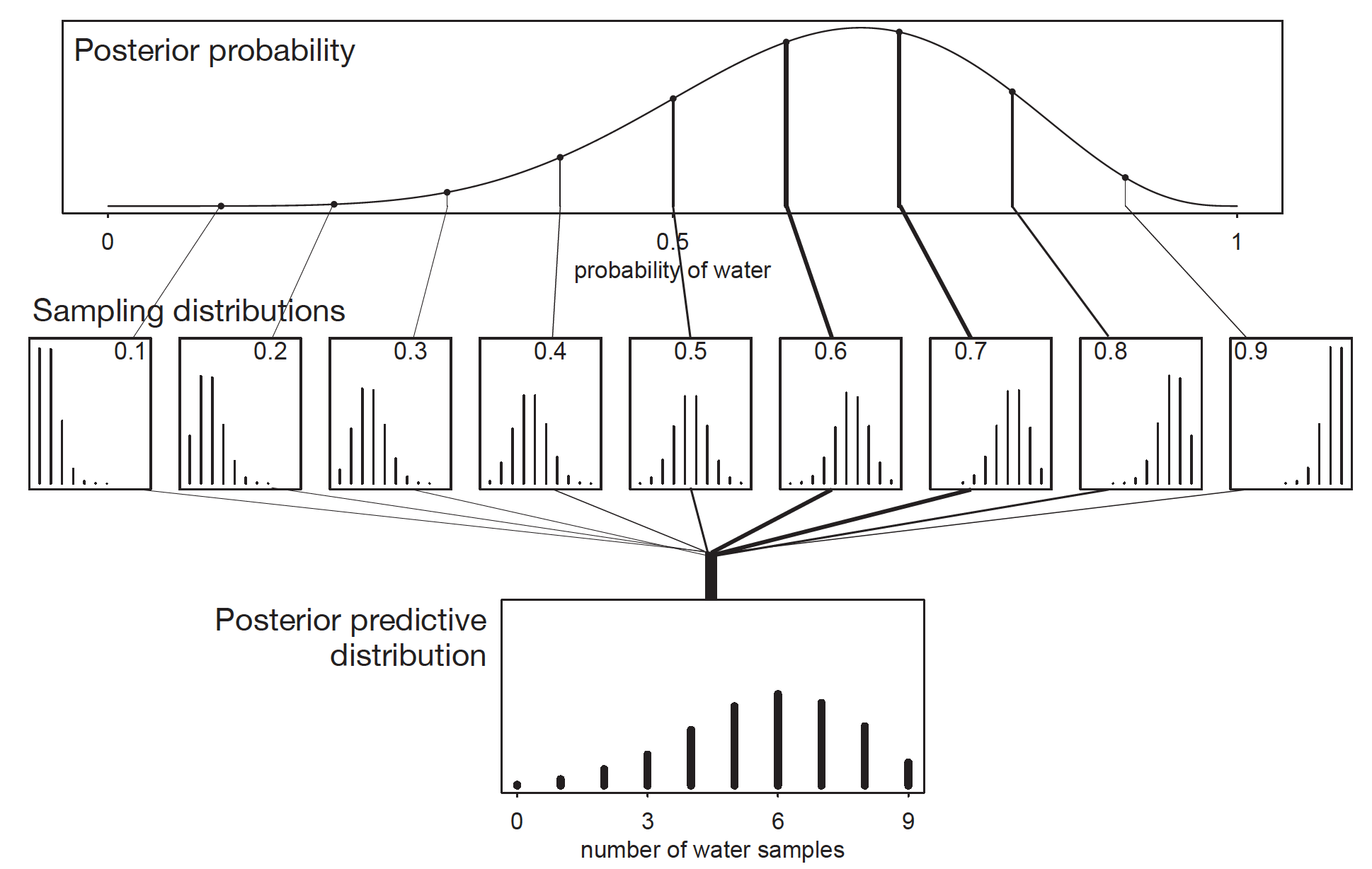
Posterior Predictive Distribution. Image from Statistical rethinking: A Bayesian course with examples in R and Stan by Richard McElreath.
w <- rbinom(1e4, size=9, prob=samples)
rethinking::dens(w, adj=2.5)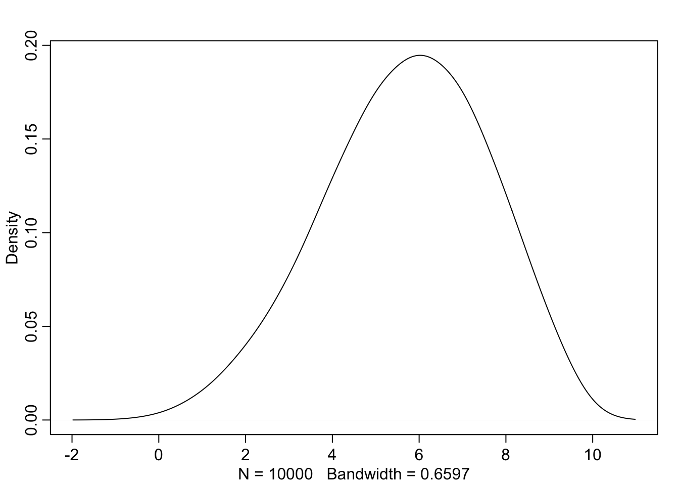
Model fitting remains an objective procedure—everyone and every golem conducts Bayesian updating in a way that doesn’t depend upon personal preferences. But model checking is inherently subjective, and this actually allows it to be quite powerful, since subjective knowledge of an empirical domain provides expertise. Expertise in turn allows for imaginative checks of model performance. Since golems have terrible imaginations, we need the freedom to engage our own imaginations. In this way, the objective and subjective work together.
References
McElreath, R. (2016). Statistical rethinking: A Bayesian course with examples in R and Stan. Chapman & Hall/CRC Press.
Kurz, A. S. (2018, March 9). brms, ggplot2 and tidyverse code, by chapter. Retrieved from https://goo.gl/JbvNTj